
Contents
- Introduction
- Why is Demand Forecasting Needed?
- Business Impact of Good Forecasting
- Time Series Data: The Foundation of Forecasting
- Real-World Data Challenges
- LSTM: The Backbone of Modern Forecasting
- Steps to Forecast with LSTM
- Dataset Overview
- Step 2: Basic preprocessing on the data:
- Step 3: Perform EDA to explore the data and visualize the data
- Conclusion
Introduction
In today’s
hyper-competitive business landscape, understanding and predicting customer
demand has become more crucial than ever. Effective demand forecasting enables
businesses to make informed decisions regarding inventory management, supply
chain operations, production schedules, and financial planning. However, the
real-world data involved in forecasting is often complex and riddled with
challenges, requiring robust preprocessing, feature engineering, and advanced
algorithms to ensure accuracy.
As Rob J. Hyndman,
a prominent statistician, notes, “Good forecasts lead to good decisions, and
good decisions can lead to success.” This highlights the vital role of accurate
forecasting in modern business.
This blog will walk
you through the process of product demand forecasting using Long Short-Term
Memory (LSTM) networks; a powerful deep learning technique ideal for time
series data. We will explore real-world data challenges, preprocessing steps,
feature engineering, and how LSTMs can unlock actionable insights for your
business.
Why is Demand Forecasting
Needed?
Accurate demand
forecasting is essential for businesses to:
- Optimize Inventory
Levels: Prevent understocking and
overstocking, both of which can have financial consequences.
- Enhance Customer
Satisfaction: Meet customer expectations by
ensuring product availability.
- Reduce Operational
Costs: Avoid unnecessary expenses in storage,
logistics, and production.
- Improve
Decision-Making: Facilitate data-driven
decisions across departments such as procurement, marketing, and sales.
To quote futurist
Peter Drucker, “The best way to predict the future is to create it.” Demand
forecasting empowers businesses to shape their strategies and operations to
align with market trends.
For instance, a
retailer who overestimates demand might overstock, leading to excessive
inventory holding costs, while underestimating demand can result in lost sales
opportunities and unhappy customers.
Business Impact of Good
Forecasting
A well-implemented
demand forecasting system can drive significant improvements in business
performance:
● Higher Revenue: By aligning stock with demand trends, businesses can capitalize on sales opportunities.
● Cost Savings: Efficient inventory management reduces waste and unnecessary expenditures.
● Better Resource Allocation: Accurate forecasts allow for optimal utilization of human and capital resources.
● Strategic Planning: Enables long-term planning for market expansions, product launches, and budget allocations.
As Steve Jobs
famously said, “You can’t connect the dots looking forward; you can only
connect them looking backward.” Forecasting helps businesses connect those dots
by analyzing past trends to anticipate future outcomes.
Conversely, poor
forecasting can lead to supply chain disruptions, strained customer
relationships, and financial losses.
Time Series Data: The
Foundation of Forecasting
Time series data
represents observations recorded sequentially over time. Examples include daily
sales, monthly revenue, or weekly website traffic. Unlike regular data, time
series has temporal dependencies, meaning past observations influence future
values. This characteristic makes it a perfect candidate for specialized
forecasting techniques like LSTM networks.
Key Characteristics of Time Series Data:
● Trend: A long-term increase or decrease in data values.
● Seasonality: Regular patterns or cycles occurring at specific intervals.
● Noise: Random variations that do not follow any identifiable pattern.
Real-World
Data Challenges
Real-world data
rarely comes clean or ready for analysis. Challenges include:
● Missing Values: Incomplete data can distort analysis.
● Outliers: Extreme values can skew predictions.
● Seasonal and Cyclical Trends: Complex patterns require careful handling.
● Stationarity: Non-stationary data, where statistical properties change over time, complicates modeling.
LSTM: The Backbone of
Modern Forecasting
Long Short-Term
Memory (LSTM) networks are a type of recurrent neural network (RNN) designed to
capture long-term dependencies in sequential data. Unlike traditional methods,
LSTMs can:
●
Handle large amounts of data
efficiently.
●
Capture complex temporal
relationships, trends, and seasonality.
●
Mitigate issues like vanishing
gradients during training.
How LSTMs Work: LSTMs use a system of
gates (input, forget, and output gates) to regulate the flow of information,
ensuring relevant patterns from the past are retained while irrelevant ones are
discarded.
Steps to Forecast with
LSTM
- Data Preparation: Split the dataset into training, validation, and test sets.
Normalize the data.
- Model Architecture: Design an LSTM model with suitable layers and hyperparameters.
- Training: Train the model on historical data using backpropagation.
- Evaluation: Use metrics like RMSE, MAE, or MAPE to assess model
performance.
- Forecasting: Generate predictions and interpret results to drive business
decisions.
Dataset Overview
Dataset I used for blog is taken from kaggle. The dataset contains historical product
demand data for a manufacturing company with a global footprint. This company
offers thousands of products across dozens of categories and operates four
central warehouses, each responsible for fulfilling regional demands. The
company manufactures its products at various locations worldwide, which means
it typically takes over a month to ship products via ocean freight to different
warehouses.
If accurate forecasts can be made for each product’s demand at these
warehouses on a monthly basis; specifically for the month after next; it could
lead to significant benefits for the company, including optimized inventory
management, reduced shipping costs, and improved customer satisfaction.
This dataset consists of five key variables:
● Product_Code: Unique identifier for each product.
● Warehouse: The central warehouse responsible for fulfilling the order.
● Product_Category: The category to which the product belongs.
● Date: The date of the order.
● Order_Demand: The quantity of demand for the product.
Steps to perform demand
forecasting
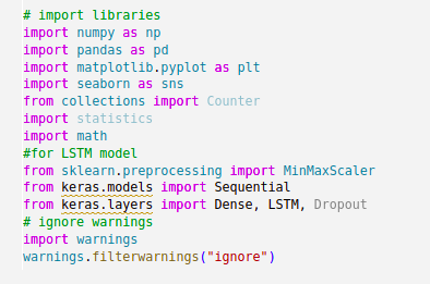
Step1: Import libraries and read the data

Step 2: Basic
preprocessing on the data:
●
Test for null and missing data
and drop them.
●
Outlier detections and handle
them with utmost care.
●
Augmented Dickey-Fuller (ADF)
test is used to check for stationarity. If the series is non-stationary, apply
transformations like differencing or detrending to make it stationary.
●
Use moving averages to smooth
the time series and reduce noise. This can help in identifying trends more
clearly.
●
If your data is in a
high-frequency format (e.g., hourly), you might want to resample it to a lower
frequency (e.g., daily or weekly) to reduce noise and make patterns more
apparent.
●
Sort the data as per the date
related information
Step 3: Perform EDA to
explore the data and visualize the data
●
Below graph depicts the count of samples according to Product
Category

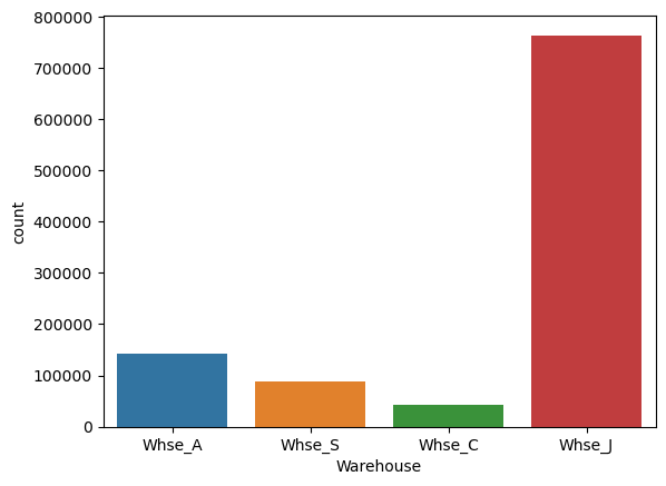
●
Below graph shows count of samples according to Warehouse
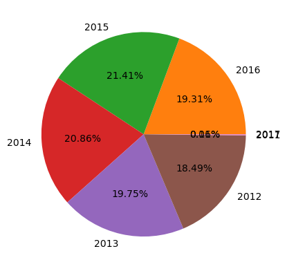
●
Percentages of Order Demand according to the years can be depicted
as under.
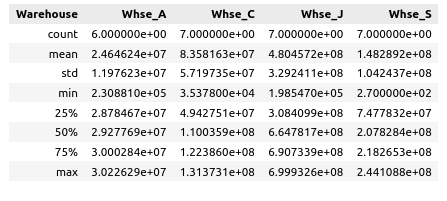
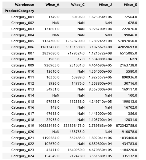
● Extraction of statistical information about warehouse data
● Each product category vs various warehouse based analysis can be given as under
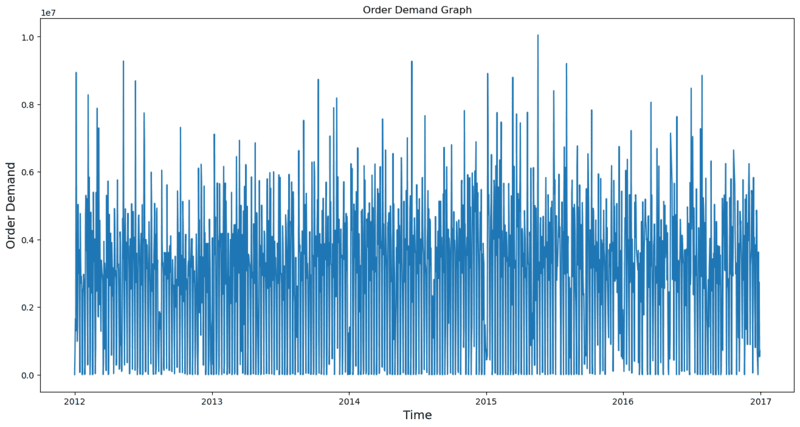
●
We can finally ensure and visualize the data as time series as
under
Step 4: Build LSTM model
The model is built using
the Keras Sequential API, enabling a straightforward stacking of layers. The
model begins with a Bidirectional LSTM layer consisting of 128 units. This
layer processes input sequences in both forward and backward directions, enhancing
the ability to understand complex temporal dependencies in the data. To prevent
overfitting, a Dropout layer is applied, randomly deactivating 20% of the
neurons during training. A second Bidirectional LSTM layer with 64 units
follows, refining the features and outputting a single value since return_sequences is set to False. Another Dropout layer is
added to regularize the network further. Following the LSTM layers, the model
includes a Dense layer with 32 neurons and a ReLU activation function,
introducing non-linearity to help extract more meaningful patterns from the data.
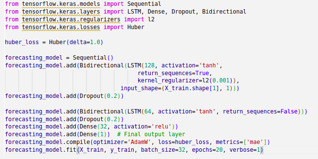
The final output layer is a
single neuron, responsible for producing the prediction, typically a regression
value. The model is compiled with the Huber loss function, known for its
robustness against outliers by combining the benefits of Mean Squared Error
(MSE) and Mean Absolute Error (MAE). It employs the AdamW optimizer, an
improved version of Adam with decoupled weight decay for better generalization,
and uses Mean Absolute Error (MAE) as the evaluation metric. After carrying out
many experiments it is concluded that the combination of Bidirectional LSTMs,
Dropout, and robust loss functions makes the model highly effective for
extracting meaningful patterns while maintaining resilience against overfitting
and noisy data.
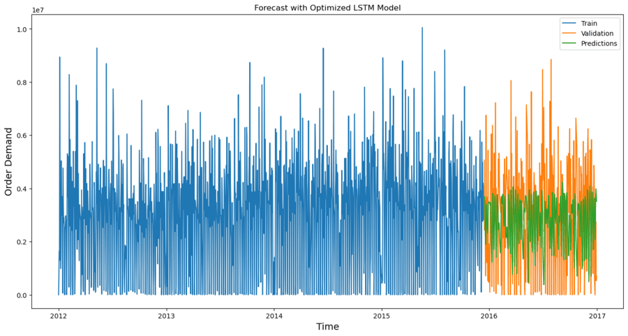
Step 5: Visualize the forecast with LSTM Model
Conclusion
Product demand
forecasting is more than just a numbers game—it’s a strategic tool that can
make or break a business. By leveraging the power of LSTMs, businesses can
unlock the full potential of their time series data, making predictions that
are not only accurate but also actionable. While challenges exist, a robust
framework involving data preprocessing, feature engineering, and LSTM modeling can
overcome them and deliver impactful results.
As renowned
physicist Niels Bohr remarked, “Prediction is very difficult, especially if
it’s about the future.” Yet, with the right tools and methods, businesses can
navigate uncertainty and seize opportunities with confidence.
Ready to transform your business with better demand forecasting? Connect with us to get more details and improved methods for improvements.